Introduction

To solve optimally the problems in science engineering, many works have been proposed to study the stability for the nonlinear system [1]. Different strong scheme have been established to solve the nonlinear problems as, Adomian Decomposition Method (ADM) [2-8], Laplace transform combined with Padé approximation [9-14], Padé Sumudu Adomian Decomposition Method (PSADM) [15] homotopy perturbation method [16,17] Modified decomposition method [18-20] have been obtained to approximate the analytical solutions. In the present paper, we analyze the behaviour of the Padé Sumudu Adomian Decomposition Methods solution (PSADM) [15] in the case of nonlinear Schrödinger equations [21] and KdV-Burgers Equations [22]. It can be seen in many literatures that the Sumudu Adomian Decomposition Methods (SADM) and Laplace Adomian Decomposition Methods (LADM) give similar results, the Sumudu transform present some advantage in calculation because have unit preserving properties (S[1] = 1). The Padé approximations have been used to control the convergence of the series solution. The function P_[L/M][.], called double Padé approximation [15] can also be use for Laplace Adomian decomposition method, and obtain the new solution. In this paper we analyze the behaviour of the Padé Sumudu Adomian Decomposition Methods Solution and provided some criteriums for the choice of the best PSADMs.

Padé Approximation

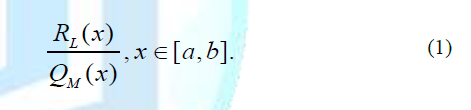
The [L,M]-order Padé approximation of the function f denote by P_x^[L,M] [f], is the quotient of two polynomials R_L(x) and Q_M(x) of degrees L and M, respectively:                   

Remark 1: The [L,M]-order Padé approximation of the function f(x) is in the form:

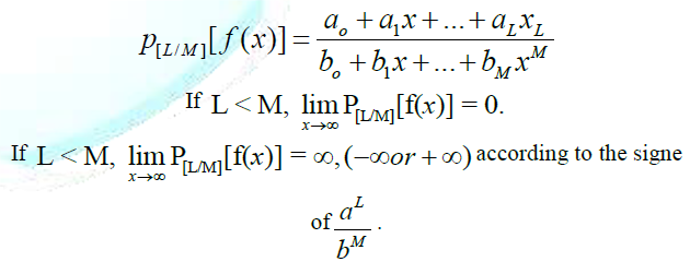
If according to the signe of .

Definition 1: Let f be function of two variables x and t. We defined two dimensional Padé approximation P_[L/M][f](x,t) of the function f as

P_[L/M] [f] (x,t) = P_x^[L,M] [P_t^[L,M] [f]] (x,t),                         (2)

where P_t^[L,M] [f] (x, t) denote the [L,M]-order Padé approximation of f(x, t) with respect to the variable t, and P_x[L,M] [f] (x, t) denote the [L,M]-order Padé approximation of f(x, t) with respect to the variable x.

If M=L, we will denote the diagonal Padé approximation of order M by P_[M/M] [f] (x, t), and called [M,M]-order Padé approximation or M Padé approximation of f(x, t).

PSADM Procedure [15]

By replacing the Sumudu transform by Laplce transform and using the same procedure we will obtain the Laplace Adomian Decomposition Methods instead of Sumudu Adomian decomposition method. 

We consider the PDE in the form as following:

L_tu(x,t)+L_xu(x,t)+R(u(x,t))+G(u(x,t))=F(x,t)             (3)

with u(x,0)=h(x) the initial condition, Lx the highest order differential respect to x, L_t the first order differential respect to t, G(u(x,y)) is the nonlinear term, F(x,t) is the inhomogeneous term, and R the remaining linear terms of lower order derivative. 

The procedure of PSADM for solving (3) can be write as follows. 

Step 1: Take the Sumudu transform to the equation (3) and apply the differentiation property of Sumudu transform to obtain 

S_t[u(x,t)](v)=h(x)+v.S_t[-L_xu(x,t)-R(u(x,t))-G(u(x,t))+F(x,t)](v).  (4) 

Step 2: Apply the inverse of the Sumudu transform to the above equation to obtain 

u(x,t)=S_v^-1[h(x)](t)+S_v^-1[v.St[-L_xu(x,t)-R(u(x,t))-G(u(x,t))+F(x,t)](v)](t)..     (5)

Step 3: Use Adomian decomposition method to decomposite the nonlinear function G(u) and the u, respectively, as

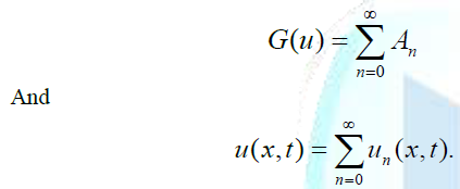
Step 4: Write the equation in the form

which lead to the SADM recursive relations:

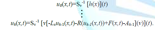
Step 5: Deduct the SADM approximation solution u_SADM=u(x,t,j):

                                u(x,t,j)=_u0+u₁+…+ uj. 

Step 6: The [L,M]-order PSADM solution uPSADM=u(x,t,j,[L,M]) is given by

                  u(x,t,j, [L,M])=P[L/M] [u_SADM] (x,t),

if L=M, we denote M-PSADM solution by

                  u(x,t,j,M)=P_[M/M] [u_SADM] (x,t). 

Remark 2: In step 5 we obtain the Sumudu Adomian Decomposition Method (SADM), instead of Sumudu transform we can use other integral transform like Laplace transform to obtain in step 5 the Laplace Adomian Decomposition Method (LADM). The Sumudu Adomian Decomposition Method and Laplace Adomian Decomposition Methods give similar result. The Sumudu transform due to the unit preserving properties (S(1)=1, provided some advantages in calculation. 

For different type of Padé approximation and different order of the Padé approximation we will analyse the behaviour of the PADM solutions.

Example 1 

In the first case of the following example, we will show that for different type of Padé approximation:

u(x, t, j, [L,M]) , for L > M,

u(x, t, j, [L,M]), for L = M, and

u(x, t, j, [L,M]), for L < M, we have different solutions and one of them is more accurate.
 

In the second case of the following example, we will show that for diagonal Padé approximation u(x,t,j, [L,M]), for L = M, we can increase the accuracy of the method by increasing or reducing de value of M accordingly to the topologie of the solution. 

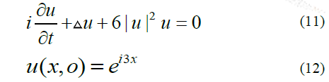
Case 1: Consider the equation:

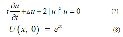
We can easily deduice the SADM solution [15]:

The algorithm is coded by the symbolic computation software Mathematica. We know u(x,t) = e^i(x+t) is the exact solution for the Problem.

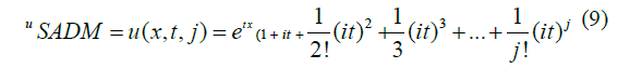
Figure (1a) and Figure (1b) show the real part and imaginary part of SADM solution u_SADM = u(x,t,15) in Domain D = [0,2] × [0,2].

For different values of L and M we plot different orders of the PSADM solutions to see the behaviour of the methods.

Figure (1c) and Figure (1d) show respectively, the real part and imaginary part of PSADM solution u_PSADM = u(x,t,15,[7,0]) in Domain D = [0,2] × [0,2].

Figure (1e) and Figure (1f) show respectively, the real part and imaginary part of PSADM solution u_PSADM = u(x,t,15,[1,7]) in Domain D = [0,2] × [0,2].

Figure (2a) and Figure (2b) show respectively, the real part and imaginary part of PSADM solution u_PSADM = u(x,t,15,[7,1]) in Domain D = [0,2] × [0,2].

Figure (2c) and Figure (2d) show respectively, the real part and imaginary part of PSADM solution u_PSADM = u(x,t,15,[7,7]) or in short u(x,t,15,7) in Domain D = [0,2] × [0,2].

Figure (2e) and Figure (2f) show the real part and imaginary part of the exact solution u(x,t) in Domain D = [0,2] × [0,2].

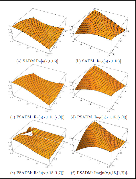
Figure 1: SADM and PSADM solutions using 15 terms.

Figure 2: (a)-(d) PSADM solutions using 15 terms, (e) and (f) exact solutions.

In domain D = [0, 2] × [0, 2] we can see that the u(x, t, 15, [1, 7]) and u(x, t, 15, [7, 1]) are not smooth compare to the other solutions. Next we plots the absolute errors.

Figure (3a) and Figure (3b) show respectively the absolute error for real part and imaginary part of the Sumudu Adomian Decomposition solution u(x, t, 15).

Figure (3c) and Figure (3d) show respectively the absolute error for real part and imaginary part of the Padé Sumudu Adomian Decomposition solution u(x, t, 15, [7, 0]).

Figure (3e) and Figure (3f) show respectively the absolute error for real part and imaginary part of the Sumudu Adomian Decomposition solution u(x, t, 15).

Now let see the behaviour of the SADM, PSADM solutions in domain D = [0, 10] × [0, 10].

Figure (4a) and Figure (4b) show the real part and imaginary part of SADM solution u_SADM = u(x, t, 15) in Domain D = [0, 10] × [0, 10].

Figure (4c) and Figure (4d) show respectively, the real part and imaginary part of PSADM solution u_PSADM = u(x, t, 15, [7, 0]) in Domain D = [0, 10] × [0, 10].

Figure (4e) and Figure (4f) show respectively, the real part and imaginary part of PSADM solution u_PSADM = u(x, t, 15, [1, 7]) in Domain D = [0, 10] × [0, 10].

Figure (5a) and Figure (5b) show respectively, the real part and imaginary part of PSADM solution u_PSADM = u(x, t, 15, [7, 1]) in Domain D = [0, 10] × [0, 10].

Figure (5c) and Figure (5d) show respectively, the real part and imaginary part of PSADM solution u_PSADM = u(x, t, 15, [7, 7]) or in short u(x, t, 15, 7) in Domain D = [0, 10] × [0, 10].

Figure (5e) and Figure (5f) show the real part and imaginary part of the exact solution u(x, t) in Domain D = [0, 10] × [0, 10].

Figure 3: Absolute errors.

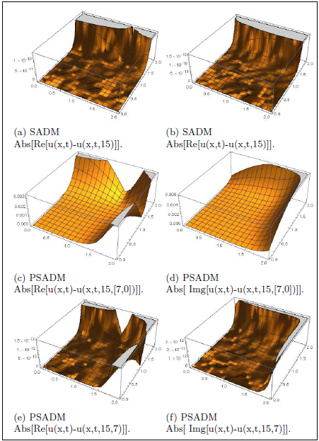
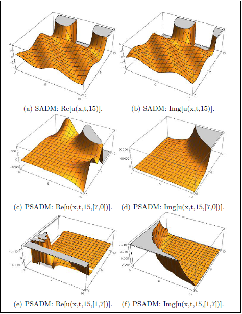
Figure 4: SADM and PSADM solutions using 15 terms.

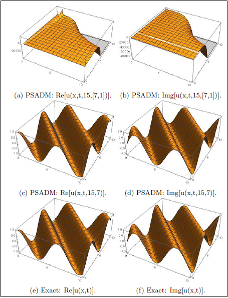
Figure 5: (a)-(d) PSADM solutions using 15 terms, (e) and (f) exact solutions.

We can see in this example, in domain D = [0, 2] × [0, 2] the SADM behave well, but in domain D = [0, 10] × [0, 10] the SADM give bad result. Only the u(x, t, 15, 7) approaching well the exact solution in the domain D = [0, 2] × [0, 2] and D = [0, 10] × [0, 10]. Even in domain

D = [0, 2] × [0, 2] the graph of absolute error show the [7, 7]-order PSADM (in short 7-PASDM) solution is better than SADM solution and other type of PSADM solutions. The solution can be perfom by choosing different value of M.

Remark 3

The real part and imaginary part of the exact solution are bounded,

and the real part and imaginary part of the SADMs are not bounded, in this case in better to use diagonal Padé approximatin to make bounded the Approximate solution. 

Case 2: Consider the equation:

We can easily deduce the SADM solution [15]:

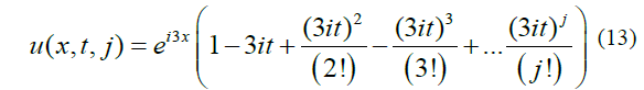
And the [L,M] order PSADM solution:

u_PSADM = u(x, t, j, [L,M]) = P_[L/M] [u(x, t, j)] (x, t),             (14)

The algorithm is coded by the symbolic computation software Mathematica.

We know u(x, t) = e^3i(x-t) is the exact solution of the Problem.

Figure (6c) and Figure (6d) show respectively the absolute error for real part and imaginary part of the PSADM solution u(x, t, 20, 7).

Figure (6e) and Figure (6f) show respectively the absolute error for real part and imaginary part of the PSADM solution u(x, t, 20, 8).

Figure (6a) and Figure (6b) show respectively the absolute error for real part and imaginary part of the SADM solution u(x, t, 20).

Figure 6: Absolute error.

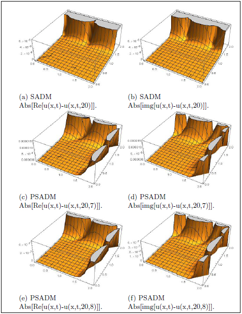
The graph of the absolute errors show that the SADM solution give better approximation than 7-order PSADM solution, and the 8-order PSADM solution give better approximation than SADM solution. The solution can be perform by choosing different value of M.

Example 2

Case 1: Consider the equation:

 Using the SADMs, we can deduice:

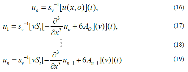
 The solution is given by:

The Sumudu Adomian Decomposition solution is given by

Then the [M,N]-oder Padé Sumudu Adomian Decomposition solution is given by

By using the symbolic computation software Mathematica.

The figure (7a), Figure (7b), Figure (7c) and Figure (7d) show respectively the curve of SADM solution u(x, t, 3), PSADM solution u_PSADM = u(x, t, 3, [2,2]), u_PSADM = u(x, t, 3, [1, 2]) and the exact solution u = u(x, t), in domain D = [-0.5, 0.5] × [0, 0.1]. The exact solution is given by u(x, t) = -2sech²(x-4t)

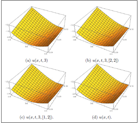
Figure 7: (a) SADM solution, (b) and (c) PSADM solutions using 3 terms, (d) exact solutions.

Figure (8a), Figure (8b), Figure (8c) and Figure (8d) show respectively the curve of SADM solution u(x, t, 3), PSADM solution u_PSADM = u(x, t, 3, [1, 2]) and the exact solution u = u(x, t), in domain D = [-1, 1] × [0, 1]

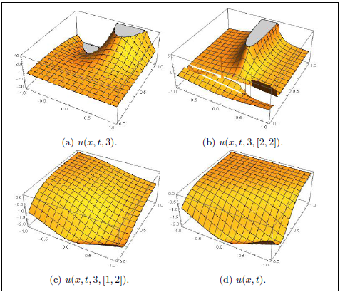
Figure 8: (a) SADM solution, (b) and (c) PSADM solutions using 3 terms, (d) exact solutions.

We can see the SADM, [2, 2]- order PSADM and [1, 2]-order PSADM solutions behave well in domain D = [-0.5, 0.5] × [0, 0.1], but only [1, 2]-order PSADM solution give better result in domain D = [-1, 1] × [0, 1]. The [2, 2]-order PSADM solution in this case in not better than [1, 2]-order PSADM solution. Then the diagonal Padé approximation are not accurate in this case. It is recommended in case to use [M,N]-order Padé approximation with M ≠ N.

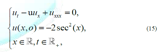
Case 2: Consider the equation:

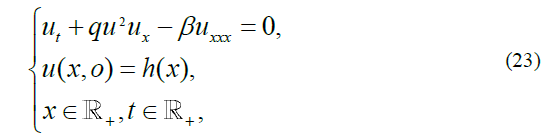
We know for q = 6, β = -1, and subject to the initial condition

the exact solution is given by:

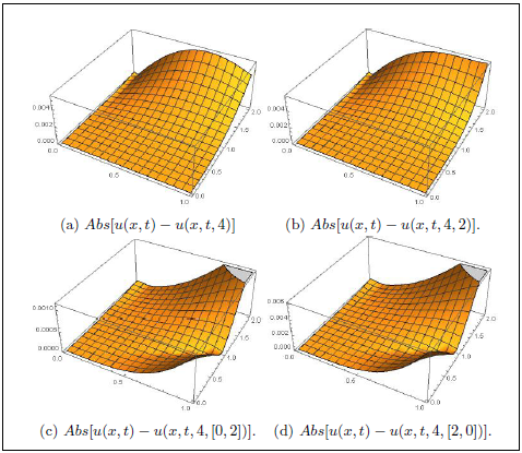
For k = 0,5, the figure (9a), Figure (9b), Figure (9c), Figure (9d), and Figure (9e) show respectively the curve of the SADM solution uSADM = u(x, t, 4), PSADM solutions u(x, t, 4, 2), u(x, t, 4, [0, 2]), u(x, t, 4, [2, 0]) and the exact solution u_exact in domain D = [0,1] × [0, 2]

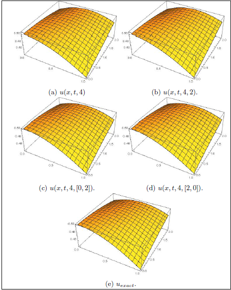
Figure 9: (a) SADM solution, (b) and (d) PSADM solutions using 4 terms, (e) exact solutions.

For k = 0.5, the figures (10a), (10b), (10c), and (10d) show respectively the absolute error curve for the SADM solution u_SADM = u(x,t,4), PSADM solutions u(x,t,4,2), u(x,t,4,[0,2]), and u(x,t,4,[2,0]) in domain D = [0,1] × [0,2] 

The SADM and [2, 2]-order PSADM (or in short 2-PSADM) provide same results. The [0, 2]-order PSADM solution in this case providing better error than [2, 2]-order PSADM and [2, 0]-order PSADM solutions. The diagonal Padé approximations are not recommended in this case.

Remark 4

The following conditions can help to choose the best PSADM solution.

Condition (*)

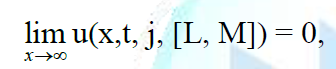
If

Figure 10: Absolute errors.

We comput the new solution by

u(x, t, j, [L,M]) = P_[L/M] [u_SADM] (x, t),with L < M

Then

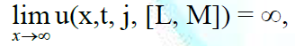
Condition (**)

If

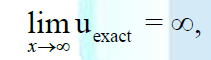
We comput the new solution by 

u(x, t, j, [L,M]) = P_[L/M] [u_SADM] (x, t),with L >M

then 

Condition (***)

If we are not in the case mentioning in conditions (*) and (**), we comput the new solution by 

u(x, t, j, [M,M]) = u(x, t, j, M) = P_[M/M] [u_SADM] (x, t),with L = M

Conclusion

In this work, we show the behaviour et of the function P_[L/M][.](x, t) using to obtain the Padé Sumudu Adomian Decomposition Methods solution for nonlinear partial differential equations such as the Schrödinger equations, and the KdV-Burger's equations. The proposed function provide us a suitable way for controlling the convergences of series solutions with high accuracy by using different order of Padé approximation and different type of the Padé approximation according to the topology of the exact solution u(x, t) and the topology of the SADM solution u(x, t, j). When the exact solutions are unknown, we have some mathematical approach to obtain more information about the topology of the exact solution. This approach can be generalized to investigate more complicated nonlinear partial differential equations that can only be solved by numerically.

Acknowledgement

This research is partially supported by the Foundations of China (Nos. 12071261, 12001539, 11831010, 11871068), the Science Challenge Project (No. TZ2018001), and the national key basic research program (No. 2018YFA0703903). The first author also acknowledges the financial support of the Chinese Scholarship Council (CSC) in Shandong University with grand (CSC No: 2020DFJ001523).

References

 1. Edwin K and Shi Y. Hopf bifurcation in three-dimensional based on Chaos Entanglement function (2019) Chaos Solitons Fractals X 4: 348-354. https://doi.org/0.1016/j.csfx.2020.100027 

2. Gabet L. The Theoretical Foundation of the Adomian Method (1994) Computers Math Appl 27: 41-52. https://doi.org/10.1016/0898-1221(94)90084-1 

3. Paripour M, Hajilou E, Hajilou A and Heidari H. Application of Adomian decomposition method to solve hybrid fuzzy differential equations (2015) Sci Direct 9: 95-103. https://doi.org/10.1016/j.jtusci.2014.06.002 

4. Muhammed Belgacem BF and Abdullatif Karaballi A. Sumudu transform fundamental properties investigations and applications (2006) J App Math Stochastic Anal 91083: 1-23. https://doi.org/10.1155/JAMSA/2006/91083

5. Kang MS, Iqbal Z, Habib M and Nazeer W. Sumudu Decomposition Method for Solving Fuzzy Integro-Differential Equations (2019) Axioms 8: 74. https://doi.org/10.3390/axioms8020074 

6. Eltayeb H, KJlJman A and Mesloub S. Application of Sumudu Decomposition Method to Solve Nonlinear System Volterra Integro-differential Equations (2014) Abstract App Anal 503141. https://doi.org/10.1155/2014/503141 

7. Manjare DN and Dinde HT. Sumudu Decomposition Method for Solving Fractional Bratu-Type Differential Equations (2014) J Sci Res 12: 585-586.https://doi.org/10.3329/jsr.v12i4.47163 

8. Hussain M and Khan M. Laplace Decomposition Method for nonlinear BURGERS-FISHERS equation (2020) Advances Math: Sci J 9: 1857-8365. https://doi.org/10.37418/amsj.9.3.60 

9. Kalateh Bojdi Z, Ahmadi-Asl S and Aminataei A. A New Extended Padé approximations and Its Application (2013) Adv Numerical Anal 2013: 263467.  https://doi.org/10.1155/2013/263467 

10. Vazquez-Leal H, Benhammouda B, Filobello-Nino U, Sarmiento-Reyes A, Jimenez-Fernandez MV, et al. Direct application of Padé approximant for solving nonlinear differential equations (2014) SpringerPlus 3: 563. https://doi.org/10.1186/2193-1801-3-563 

11. Pad H. Thesis: Representation approximative of a function by a rational function of given order (2014) Ann Sci cole Norm 3: 1-93. https://doi.org/10.1007/978-3-642-58169-4 

12. Baker GA. The existence and convergence of subsequences of Padé approximants (1973) J Math Anal Appl 43: 498-528. https://doi.org/10.1016/0022-247X(73)90088-7 

13. Richard M and Zhao W. Padé-Sumudu-Adomian Decomposition Method for solving nonlinear Schrödinger equation (2021) J Appl Math. https://doi.org/10.1155/2021/6626236

14. Selivanov FM and Chernoivan AY. A Combined approch of the Laplace transform and Padé approximation solving viscoelasticity problem-19s (2006) Int J Solids Structures 44: 6676. https://doi.org/10.1016/j.ijsolstr.2006.04.012  

15. Kovacheva R. A note on over convergent subsequences of the mth row of classical Padé approximants (2018) AIP Conf Proceedings 2048: 050013. https://doi.org/10.1063/1.5082112

16. Al-Nemrat A and Zainuddin Z. Homotopy perturbation Sumudu transform method for solving nonlinear boundary value problems (2018) AIP Conf Proceedings. https://doi.org/10.1063/1.5041640 

17. Ganjefar S and Rezaei S. A modified homotopy perturbation method for optimal control problems using Padé approximant (2016) Appl Math Modelling 40: 15-16. https://doi.org/10.1016/j.apm.2016.02.039 

18. Ziane D, Belgacem R and Bokhari A. A new modified Adomian decomposition method for nonlinear partial differential equations (2016) Open J Math Anal. https://doi.org/10.30538/psrp-oma2019.0041 

19. Wazwaz MA and El-Sayed MS. A new modification of the Adomian decomposition method for linear and nonlinear operators (2001) Appl Math Computation 122: 393-405. https://doi.org/10.1016/S0096-3003(00)00060-6 

20. Umut O and Yaar S. Numerical Treatment of Initial Value Problems of Nonlinear Ordinary Differential Equations by Duan-Rach-Wazwaz Modified Adomian Decomposition Method (2019) Int J Modern Nonlinear Theory Applicatn 8: 90362. https://doi.org/10.4236/ijmnta.2019.81002 

21. Jaradat KE, Alomari O, Abudayah M and Al-Faqih MA. An Approximate Analytical Solution of the Nonlinear Schrödinger Equation with Harmonic Oscillator Using Homotopy Perturbation Method and Laplace-Adomian Decomposition Method (2018) Adv Math Physics 2018: 6765021. https://doi.org/10.1155/2018/6765021 

22. Benia Y and Scapellato A. Existence of solution to Kortewegde Vries equation in a non-parabolic domain (2020) Nonlinear Anal 195: 111758. https://doi.org/10.1016/j.na.2020.111758 

Corresponding author

Metonou Richard, School of Mathematics, Shandong University, China, E-mail: metonourichard@yahoo.fr

Weidong Zhao, School of Mathematics, Shandong University, China, E-mail: wdzhao@sdu.edu.cn

Citation

Keywords

Adomian Decomposition Method (ADM), Padé Sumudu Adomian Decomposition Method (PSADM), Nonlinear Schrödinger equation, Nonlinear KdV Burger's equation.